A Deep Dive in OSPF LSAs, Part 3

In my previous post I covered Type 1 and Type 2 LSAs in relation to broadcast networks. In this post I’ll demonstrate how you can use these LSAs to map the topology an OSPF area.

Broadcast Networks - Type 1 + Type 2 LSAs = Area Diagram

First, let’s take a look at which LSAs exist in this area:

R1(config-if)#do sh ip ospf database

            OSPF Router with ID (1.1.1.1) (Process ID 1)

                Router Link States (Area 0)

Link ID         ADV Router      Age         Seq#       Checksum Link count
1.1.1.1         1.1.1.1         1850        0x8000000C 0x003FB9 1
2.2.2.2         2.2.2.2         370         0x8000000D 0x00278E 2
3.3.3.3         3.3.3.3         339         0x80000004 0x0001EA 1

                Net Link States (Area 0)

Link ID         ADV Router      Age         Seq#       Checksum
10.1.2.1        1.1.1.1         823         0x80000003 0x0055C4
10.2.3.2        2.2.2.2         370         0x80000002 0x006C9F 

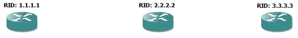
Given the Type 1 LSA’s above, we immediately know there are three routers in this area. We also know that R2 has two links, whereas R1 and R3 only have one each. By putting this information together, our diagram looks like this:

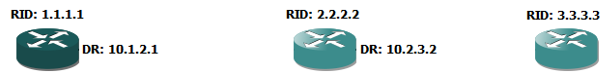
Now, given the Type 2 LSA’s above, we also know which of these routers have interfaces which are DRs. Let’s add this information to our diagram:

Let’s now analyse the Type 1 LSAs to see what information we can gather from them:

R1#sh ip os da rou

            OSPF Router with ID (1.1.1.1) (Process ID 1)

                Router Link States (Area 0)

  LS age: 44
  Options: (No TOS-capability, DC)
  LS Type: Router Links
  Link State ID: 1.1.1.1
  Advertising Router: 1.1.1.1
  LS Seq Number: 80000003
  Checksum: 0x51B0
  Length: 36
  AS Boundary Router
  Number of Links: 1

    Link connected to: a Transit Network
     (Link ID) Designated Router address: 10.1.2.1
     (Link Data) Router Interface address: 10.1.2.1
      Number of TOS metrics: 0
       TOS 0 Metrics: 10

• The output above tells us that the router with RID 1.1.1.1 has only one link, and that link’s address is 10.1.2.1. This link address (R1’s interface) is the DR for that segment.
• We already knew this from the previous output so there’s nothing new to add to the diagram just yet.

LS age: 39
  Options: (No TOS-capability, DC)
  LS Type: Router Links
  Link State ID: 2.2.2.2
  Advertising Router: 2.2.2.2
  LS Seq Number: 80000004
  Checksum: 0x3985
  Length: 48
  Number of Links: 2

    Link connected to: a Transit Network
     (Link ID) Designated Router address: 10.2.3.2
     (Link Data) Router Interface address: 10.2.3.2
      Number of TOS metrics: 0
       TOS 0 Metrics: 10

    Link connected to: a Transit Network
     (Link ID) Designated Router address: 10.1.2.1
     (Link Data) Router Interface address: 10.1.2.2
      Number of TOS metrics: 0
       TOS 0 Metrics: 10

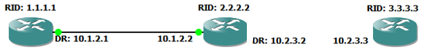
• The output above tells us that the router with RID 2.2.2.2 has two links. They are 10.2.3.2 (which RID 2.2.2.2 is the DR for) as well as 10.1.2.2 (which has a DR of 10.1.2.1).
  • We already knew about 10.2.3.2 and that it is the DR for that segment, so there’s nothing new there.
  • However, we did not know about 10.1.2.2. This is because the “show ip ospf database” command only shows us DR link addresses.
  • Now that we know about this link address and that its DR is 10.1.2.1, we know that there is a connection between the routers with RID 1.1.1.1 and RID 2.2.2.2.
  • Our diagram now looks like this:

LS age: 41
  Options: (No TOS-capability, DC)
  LS Type: Router Links
  Link State ID: 3.3.3.3
  Advertising Router: 3.3.3.3
  LS Seq Number: 80000003
  Checksum: 0x3E9
  Length: 36
  Number of Links: 1

    Link connected to: a Transit Network
     (Link ID) Designated Router address: 10.2.3.2
     (Link Data) Router Interface address: 10.2.3.3
      Number of TOS metrics: 0
       TOS 0 Metrics: 10

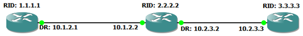
• The output above tells us that the router with RID 3.3.3.3 has only one link, and that link’s address is 10.2.3.3.
  • As was the case with RID 2.2.2.2’s link address 10.2.2.2, we didn’t know about RID 3.3.3.3’s 10.2.3.3 link address because it is not a DR, and therefore did not appear in the  ”show ip ospf database” output.
  • Now that we know about this link address and that its DR is 10.2.3.2, we know that there is a connection between the routers with RID 2.2.2.2 and RID 3.3.3.3.
  • Our diagram now looks like this:

The last remaining question is, what are the size(s) of the subnets for these links? Are they /30, /24, etc?

To answer this question we’ll need to look at the Type 2 LSAs:

R1#sh ip os da network

            OSPF Router with ID (1.1.1.1) (Process ID 1)

                Net Link States (Area 0)

  Routing Bit Set on this LSA
  LS age: 368
  Options: (No TOS-capability, DC)
  LS Type: Network Links
  Link State ID: 10.1.2.1 (address of Designated Router)
  Advertising Router: 1.1.1.1
  LS Seq Number: 80000002
  Checksum: 0x57C3
  Length: 32
  Network Mask: /24
        Attached Router: 1.1.1.1
        Attached Router: 2.2.2.2

  Routing Bit Set on this LSA
  LS age: 322
  Options: (No TOS-capability, DC)
  LS Type: Network Links
  Link State ID: 10.2.3.2 (address of Designated Router)
  Advertising Router: 2.2.2.2
  LS Seq Number: 80000002
  Checksum: 0x6C9F
  Length: 32
  Network Mask: /24
        Attached Router: 2.2.2.2
        Attached Router: 3.3.3.3

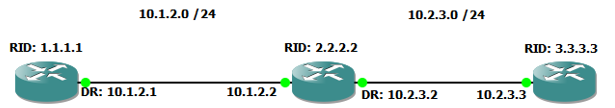
As we can see above, they’re both /24 subnets. With this final piece of information, we’ve now got a complete diagram of this area:

 Other Posts in this Series

See the A Deep Dive in OSPF LSAs - Index post for links to all of the posts in this series.

---

As always, if you have any questions or have a topic that you would like me to discuss, please feel free to post a comment at the bottom of this blog entry, e-mail at will@oznetnerd.com, or drop me a message on Reddit (OzNetNerd).

Note: The opinions expressed in this blog are my own and not those of my employer.